The covariance test

One of the first works in this framework of post-selection inference is the covariance test. The test was motivated by a drop in covariance of the residual through one step of the LARS path.

The basic theory behind the covtest can be seen by sampling $n$ IID Gaussians and looking at the spacings between the top two. A simple calculation Mills’ ratio calculation leads to

$$Z^n_{(1)} (Z^n_{(1)} - Z^n_{(2)}) \overset{D}{\to} \text{Exp}(1)$$

Here is a little simulation.

import numpy as np
np.random.seed(0)
%matplotlib inline
import matplotlib.pyplot as plt
from statsmodels.distributions import ECDF
from selectinf.algorithms.covtest import covtest

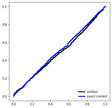
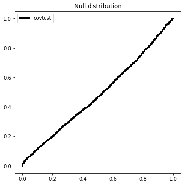
We will sample 2000 times from $Z \sim N(0,I_{50 \times 50})$ and look at the normalized spacing between the top 2 values.

Z = np.random.standard_normal((2000,50))
T = np.zeros(2000)
for i in range(2000):
    W = np.sort(Z[i])
    T[i] = W[-1] * (W[-1] - W[-2])

Ugrid = np.linspace(0,1,101)
covtest_fig = plt.figure(figsize=(6,6))
ax = covtest_fig.gca()
ax.plot(Ugrid, ECDF(np.exp(-T))(Ugrid), drawstyle='steps', c='k',
        label='covtest', linewidth=3)
ax.set_title('Null distribution')
ax.legend(loc='upper left');

The covariance test is an asymptotic result, and can be used in a sequential procedure called forward stop to determine when to stop the LASSO path.

An exact version of the covariance test was developed in a general framework for problems beyond the LASSO using the Kac-Rice formula. A sequential version along the LARS path was developed, which we refer to as the spacings test.

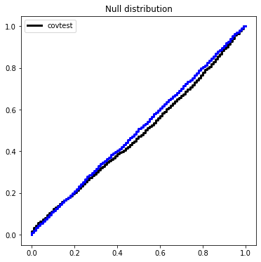
Here is the exact test, which is the first step of the spacings test.

from scipy.stats import norm as ndist
Texact = np.zeros(2000)
for i in range(2000):
    W = np.sort(Z[i])
    Texact[i] = ndist.sf(W[-1]) / ndist.sf(W[-2])
ax.plot(Ugrid, ECDF(Texact)(Ugrid), c='blue', drawstyle='steps', label='exact covTest',
        linewidth=3)
covtest_fig

Covariance test for regression

The above tests were based on an IID sample, though both the covtest and its exact version can be used in a regression setting. Both tests need access to the covariance of the noise.

Formally, suppose

$$y|X \sim N(\mu, \Sigma)$$

the exact test is a test of

$$H_0:\mu=0.$$

The test is based on

$$\lambda_{\max} = \|X^Ty\|_{\infty}.$$

This value of $\lambda$ is the value at which the first variable enters the LASSO. That is, $\lambda_{\max}$ is the smallest $\lambda$ for which 0 solves

$$\text{minimize}_{\beta} \frac{1}{2} \|y-X\beta\|^2_2 + \lambda \|\beta\|_1.$$

Formally, the exact test conditions on the variable $i^*(y)$ that achieves $\lambda_{\max}$ and tests a weaker null hypothesis

$$H_0:X[:,i^*(y)]^T\mu=0.$$

The covtest is an approximation of this test, based on the same Mills ratio calculation. (This calculation roughly says that the overshoot of a Gaussian above a level $u$ is roughly an exponential random variable with mean $u^{-1}$).

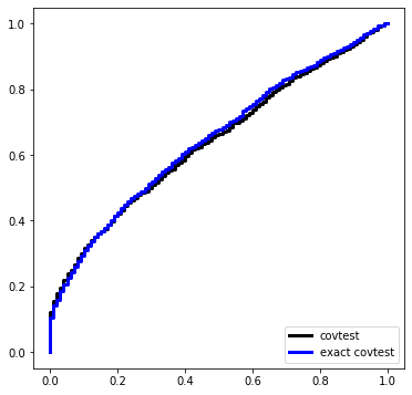
Here is a simulation under $\Sigma = \sigma^2 I$ with $\sigma$ known. The design matrix, before standardization, is Gaussian equicorrelated in the population with parameter 1/2.

n, p, nsim, sigma = 50, 200, 1000, 1.5

def instance(n, p, beta=None, sigma=sigma):
    X = (np.random.standard_normal((n,p)) + np.random.standard_normal(n)[:,None])
    X /= X.std(0)[None,:]
    X /= np.sqrt(n)
    Y = np.random.standard_normal(n) * sigma
    if beta is not None:
        Y += np.dot(X, beta)
    return X, Y

Let’s make a dataset under our global null and compute the exact covtest $p$-value.

X, Y = instance(n, p, sigma=sigma)
cone, pval, idx, sign = covtest(X, Y, exact=False)
pval

0.06488988967797554

The object cone is an instance of selection.affine.constraints which does much of the work for affine selection procedures. The variables idx and sign store which variable achieved $\lambda_{\max}$ and the sign of its correlation with $y$.

cone

$$Z \sim N(\mu,\Sigma) | AZ \leq b$$

def simulation(beta):
    Pcov = []
    Pexact = []

    for i in range(nsim):
        X, Y = instance(n, p, sigma=sigma, beta=beta)
        Pcov.append(covtest(X, Y, sigma=sigma, exact=False)[1])
        Pexact.append(covtest(X, Y, sigma=sigma, exact=True)[1])

    Ugrid = np.linspace(0,1,101)
    plt.figure(figsize=(6,6))
    plt.plot(Ugrid, ECDF(Pcov)(Ugrid), label='covtest', ds='steps', c='k', linewidth=3)
    plt.plot(Ugrid, ECDF(Pexact)(Ugrid), label='exact covtest', ds='steps', c='blue', linewidth=3)
    plt.legend(loc='lower right')

Null

beta = np.zeros(p)
simulation(beta)

1-sparse

beta = np.zeros(p)
beta[0] = 4
simulation(beta)

2-sparse

beta = np.zeros(p)
beta[:2] = 4
simulation(beta)

5-sparse

beta = np.zeros(p)
beta[:5] = 4
simulation(beta)