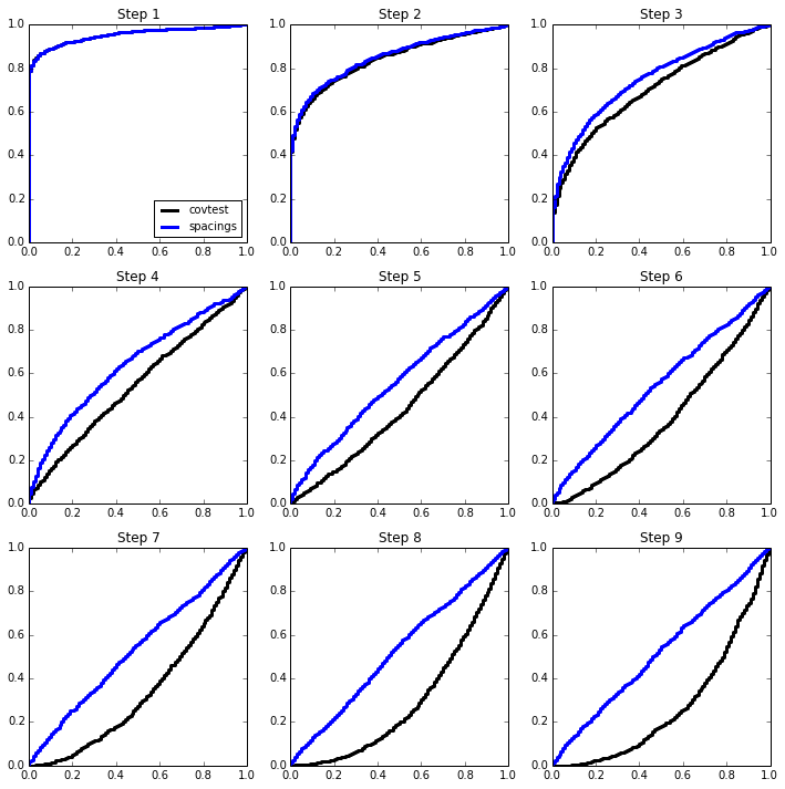
The spacings test
The covariance test describes the distribution of spacings at points on the LARS path for the LASSO (see the paper).
It is an asymptotic distribution for the “first null step” that LARS
takes. That is, if there are 5 strong variables in the model, the 6th
covtest \(p\)-value should be approximately uniform on [0,1].
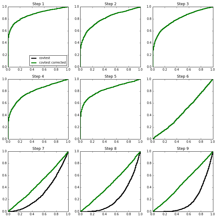
Before the 6th step, we expect (or hope) to see low p-values, but what about after the 6th step? In the paper, it is pointed out that in the orthogonal case, the subsequent steps look like Exp random variables with means depending on how far beyond the “first null” we are.
Here is an illustration of this phenomenon in the orthogonal case, for which we expect
import numpy as np
np.random.seed(0)
%matplotlib inline
import matplotlib.pyplot as plt
from statsmodels.distributions import ECDF
from selection.covtest import covtest
We will sample 2000 times from \(Z \sim N(\mu,I_{100 \times 100})\) and look at the normalized spacing between the top 2 values. The mean vector \(\mu\) will be sparse, with 5 large values.
Z = np.random.standard_normal((2000,100))
Z[:,:5] += np.array([4,4.5,5,5.5,6])[None,:]
T = np.zeros((2000,9))

for i in range(2000):
    W = np.sort(Z[i])[::-1]
    for j in range(9):
        T[i,j] = W[j] * (W[j] - W[j+1])

covtest_fig, axes = plt.subplots(3,3, figsize=(12,12))
Ugrid = np.linspace(0,1,101)
for i in range(3):
    for j in range(3):
        ax = axes[i,j]
        ax.plot(Ugrid, ECDF(np.exp(-T[:,3*i+j]))(Ugrid), linestyle='steps', c='k',
                label='covtest', linewidth=3);
        ax.set_title('Step %d' % (3*i+j+1))
        if (i, j) == (0, 0):
            ax.legend(loc='lower right', fontsize=10)
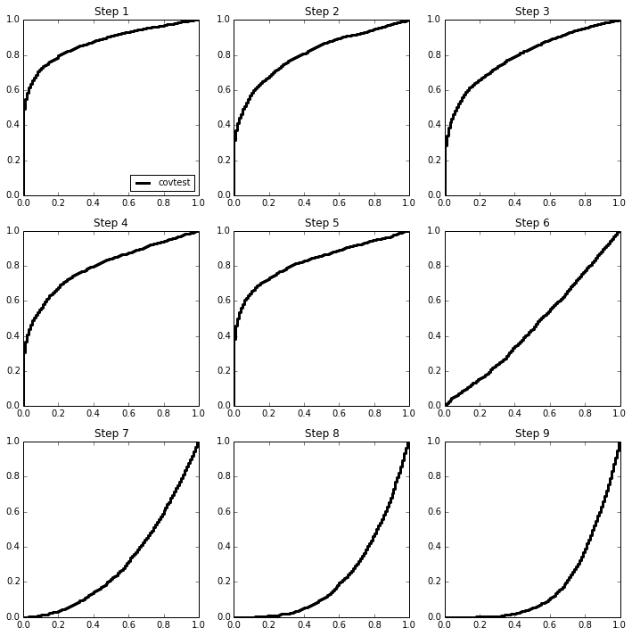
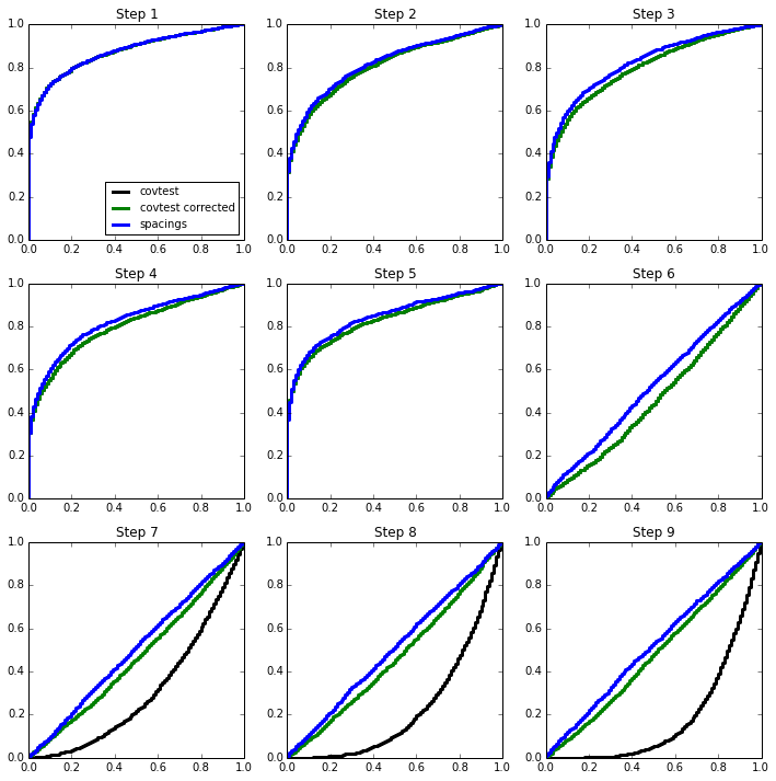
Knowing there are 5 strong signals, we can apply the approximation about the exponentials of different sizes to the later steps. The last 4 p-values now all seem roughly uniform on (0,1)
factor = np.array([1,1,1,1,1,1,2,3,4])
T *= factor

for i in range(3):
    for j in range(3):
        ax = axes[i,j]
        ax.plot(Ugrid, ECDF(np.exp(-T[:,3*i+j]))(Ugrid), linestyle='steps',
                c='green',
                label='covtest corrected', linewidth=3)
        if (i, j) == (0, 0):
            ax.legend(loc='lower right', fontsize=10)
covtest_fig
Spacings test
The `spacings test <>`__ does not show this same behaviour at later stages of the path, as it keeps track of the order of the variables that have “entered” the model.
from scipy.stats import norm as ndist
spacings = np.zeros((2000,9))

for i in range(2000):
    W = np.sort(Z[i])[::-1]
    for j in range(9):
        if j > 0:
            spacings[i,j] = ((ndist.sf(W[j-1]) - ndist.sf(W[j])) /
                             (ndist.sf(W[j-1]) - ndist.sf(W[j+1])))
        else:
            spacings[i,j] = ndist.sf(W[j]) / ndist.sf(W[j+1])

for i in range(3):
    for j in range(3):
        ax = axes[i,j]
        ax.plot(Ugrid, ECDF(spacings[:,3*i+j])(Ugrid), linestyle='steps', c='blue',
                label='spacings', linewidth=3)
        if (i, j) == (0, 0):
            ax.legend(loc='lower right', fontsize=10)
covtest_fig
Spacings in a regression setting
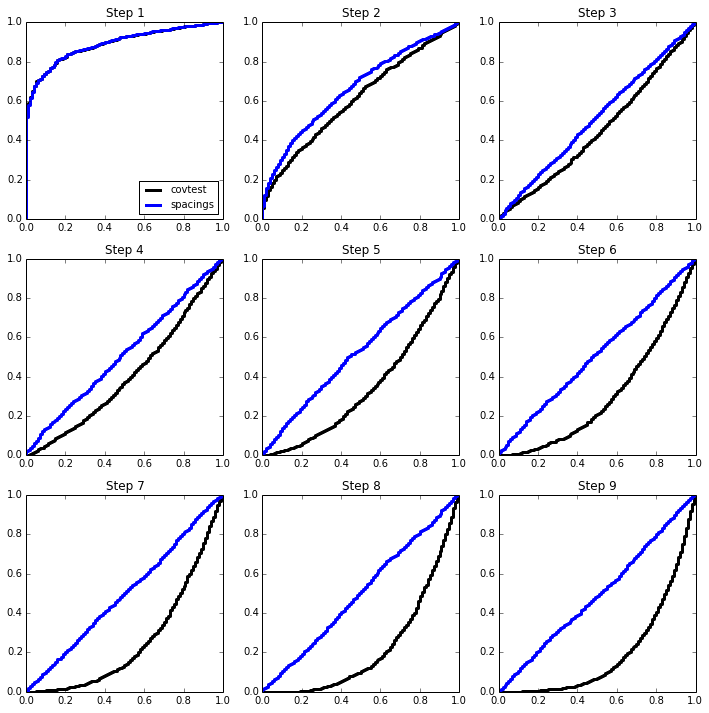
The spacings test can be used in a regression setting as well. The spacings paper describes this approach for the LARS path, though it can also be used in other contexts.
Below, we use it in forward stepwise model selection.
n, p, nsim, sigma = 50, 200, 1000, 1.5

def instance(n, p, beta=None, sigma=sigma):
    X = (np.random.standard_normal((n,p)) + np.random.standard_normal(n)[:,None])
    X -= X.mean(0)[None,:]
    X /= X.std(0)[None,:]
    X /= np.sqrt(n)
    Y = np.random.standard_normal(n) * sigma
    if beta is not None:
        Y += np.dot(X, beta)
    return X, Y
from selection.forward_step import forward_stepwise
X, Y = instance(n, p, sigma=sigma)
FS = forward_stepwise(X, Y)
for _ in range(5):
    FS.next()
FS.variables
[106, 78, 58, 135, 97]
The steps taken above should match R’s output. We first load the
%R magic.
%load_ext rmagic
Recall that R uses 1-based indexing so there will be a difference of
1 in the indexes of selected variables.
%%R -i X,Y
D = data.frame(X,Y)
model5 = step(lm(Y ~ 1, data=D), list(upper=lm(Y ~ ., data=D)), direction='forward',
     k=0, steps=5, trace=FALSE)
model5
Call:
lm(formula = Y ~ X107 + X79 + X59 + X136 + X98, data = D)

Coefficients:
(Intercept)         X107          X79          X59         X136          X98
     0.1062      -4.1047       8.2780      -6.4041       6.1924      -4.7872
Covariance test for forward stepwise
While the covtest was derived for the LASSO, it can be used
sequentially in forward stepwise as well. Consider the model
The basic approach is to note that covtest provides, a test of the
null
Subsequent steps essentially reapply this same test forgetting what has happened previously. In the case of the LARS path, each addition step can be expressed as a choice among several competing variables to add (see uniqueness and spacings for more details).
To use the covtest for forward stepwise, we orthogonalize with
respect to the variables already chosen and apply the covtest to the
residual and orthogonalized \(X\) matrix.
Specifically, denote \(R_{M[j]}\) the residual forming matrix at the
\(j\)-th step, with \(R_0=I\) with \(M[j]\) the \(j\)-th
model. At the \(j+1\)-st step, we simply compute the covtest
with design \(R_{M[j]}X\) (with normalized columns) and response
\(R_{M[j]}Y\).
from selection.affine import constraints

def forward_step(X, Y, sigma=1.5,
                 nstep=9):

    n, p = X.shape
    FS = forward_stepwise(X, Y)
    spacings_P = []
    covtest_P = []

    for i in range(nstep):
        FS.next()

        if FS.P[i] is not None:
            RX = X - FS.P[i](X)
            RY = Y - FS.P[i](Y)
            covariance = np.identity(n) - np.dot(FS.P[i].U, FS.P[i].U.T)
        else:
            RX = X
            RY = Y
            covariance = None
        RX -= RX.mean(0)[None,:]
        RX /= RX.std(0)[None,:]

        con, pval, idx, sign = covtest(RX, RY, sigma=sigma,
                                       covariance=covariance,
                                       exact=False)
        covtest_P.append(pval)

        # spacings

        eta = RX[:,idx] * sign
        spacings_constraint = constraints(FS.A, np.zeros(FS.A.shape[0]))
        spacings_constraint.covariance *= sigma**2
        spacings_P.append(spacings_constraint.pivot(eta, Y))

    return covtest_P, spacings_P
The above function computes our covtest and spacings \(p\)-values for several steps of forward stepwise.
forward_step(X, Y, sigma=sigma)
([0.73909103381622476,
  0.69360763579435791,
  0.39906919537104235,
  0.81146065359168629,
  0.55327261959262941,
  0.80265701686406743,
  0.90884645708288014,
  0.99181179452730495,
  0.64069596746441959],
 [0.694095750161889,
  0.6513481019927231,
  0.3234919672656077,
  0.573180829314827,
  0.44008971114931383,
  0.5542519955483218,
  0.8596480260839896,
  0.9073752648845056,
  0.11680940361115943])
def simulation(n, p, sigma, beta):
    covtest_P = []
    spacings_P = []

    for _ in range(1000):
        X, Y = instance(n, p, sigma=sigma, beta=beta)
        _cov, _spac = forward_step(X, Y, sigma=sigma)
        covtest_P.append(_cov)
        spacings_P.append(_spac)

    covtest_P = np.array(covtest_P)
    spacings_P = np.array(spacings_P)

    regression_fig, axes = plt.subplots(3,3, figsize=(12,12))
    Ugrid = np.linspace(0,1,101)
    for i in range(3):
        for j in range(3):
            ax = axes[i,j]
            ax.plot(Ugrid, ECDF(covtest_P[:,3*i+j])(Ugrid), linestyle='steps', c='k',
                    label='covtest', linewidth=3)
            ax.plot(Ugrid, ECDF(spacings_P[:,3*i+j])(Ugrid), linestyle='steps', c='blue',
                    label='spacings', linewidth=3)
            ax.set_title('Step %d' % (3*i+j+1))
            if (i,j) == (0,0):
                ax.legend(loc='lower right', fontsize=10)

    return np.array(covtest_P), np.array(spacings_P)
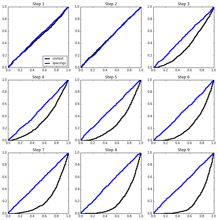
2-sparse model
beta = np.zeros(p)
beta[:2] = np.array([4,4.5]) * sigma
simulation(n, p, sigma, beta);
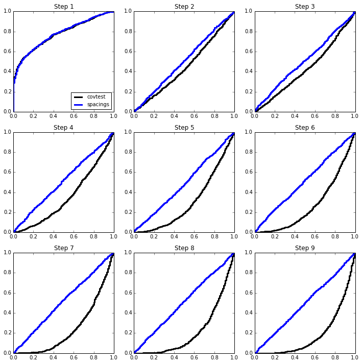
5-sparse model
beta = np.zeros(p)
beta[:5] = np.array([4,4.5,5,5.5,3.5]) * sigma
simulation(n, p, sigma, beta);
