Inference in the full model

This is the same example as considered in Liu et al. though we do not consider the special analysis in that paper. We let the computer guide us in correcting for selection.

The functions full_model_inference and pivot_plot below are just simulation utilities used to simulate results in least squares regression. The underlying functionality is contained in the function selectinf.learning.core.infer_full_target.

import functools

import numpy as np, pandas as pd
import matplotlib.pyplot as plt
%matplotlib inline
import regreg.api as rr

from selectinf.tests.instance import gaussian_instance # to generate the data
from selectinf.learning.core import normal_sampler     # our representation of the (limiting) Gaussian data

from selectinf.learning.utils import full_model_inference, pivot_plot
from selectinf.learning.fitters import gbm_fit_sk

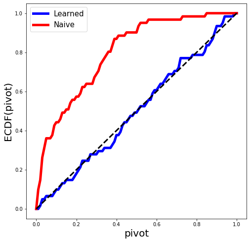
We will know generate some data from an OLS regression model and fit the LASSO with a fixed value of \(\lambda\). In the simulation world, we know the true parameters, hence we can then return pivots for each variable selected by the LASSO. These pivots should look (marginally) like a draw from np.random.sample. This is the plot below.

np.random.seed(0) # for replicability

def simulate(n=200,
             p=20,
             s=5,
             signal=(0.5, 1),
             sigma=2,
             alpha=0.1,
             B=6000,
             verbose=False):

    # description of statistical problem

    X, y, truth = gaussian_instance(n=n,
                                    p=p,
                                    s=s,
                                    equicorrelated=False,
                                    rho=0.5,
                                    sigma=sigma,
                                    signal=signal,
                                    random_signs=True,
                                    scale=False)[:3]


    XTX = X.T.dot(X)
    XTXi = np.linalg.inv(XTX)
    resid = y - X.dot(XTXi.dot(X.T.dot(y)))
    dispersion = np.linalg.norm(resid)**2 / (n-p)

    S = X.T.dot(y)
    covS = dispersion * X.T.dot(X)

    # this declares our target as linear in S where S has a given covariance
    sampler = normal_sampler(S, covS)

    def base_algorithm(XTX, lam, sampler):

        p = XTX.shape[0]
        success = np.zeros(p)

        loss = rr.quadratic_loss((p,), Q=XTX)
        pen = rr.l1norm(p, lagrange=lam)

        scale = 0.
        noisy_S = sampler(scale=scale)
        loss.quadratic = rr.identity_quadratic(0, 0, -noisy_S, 0)
        problem = rr.simple_problem(loss, pen)
        soln = problem.solve(max_its=100, tol=1.e-10)
        success += soln != 0

        return set(np.nonzero(success)[0])


    lam = 3.5 * np.sqrt(n)
    selection_algorithm = functools.partial(base_algorithm, XTX, lam)
    if verbose:
        print(selection_algorithm(sampler))
    # run selection algorithm

    return full_model_inference(X,
                                y,
                                truth,
                                selection_algorithm,
                                sampler,
                                success_params=(1, 1),
                                B=B,
                                fit_probability=gbm_fit_sk,
                                fit_args={'n_estimators':500})

Let’s take a look at what we get as a return value:

while True:
    df = simulate(verbose=True)
    if df is not None:
        break
df.columns

{19}

Index(['B', 'alpha', 'coverage', 'id', 'length', 'lower', 'nfeature',
       'nsample', 'pivot', 'pvalue', 'target', 'upper', 'variable',
       'bonferroni_coverage', 'bonferroni_length', 'bonferroni_lower',
       'bonferroni_pvalue', 'bonferroni_upper', 'naive_coverage',
       'naive_length', 'naive_lower', 'naive_pivot', 'naive_pvalue',
       'naive_upper'],
      dtype='object')

dfs = []
for i in range(30):
    df = simulate()
    if df is not None:
        dfs.append(df)

fig = plt.figure(figsize=(8, 8))
results = pd.concat(dfs)
pivot_plot(results, fig=fig);